Introduction and Motivation


After the creation of President Obama's 2015 Task Force on 21st Century Policing, many police departments pushed to implement community focused policing tactics. This meant creating a more comprehensive support system for the community that focused on holistic public health rather than arrests and conviction numbers. As an extension of this, our team decided to look into Analyze Boston's police report dataset, which included records of all police reports filed from 2015 to 2019. We wanted to analyze police reports to see what sort of emergency responses correlated with different location, neighboorhood-attribute, time, and weather predictors. For example, if we could predict 911 calls that had a high likelihood of involving domestic abuse, then we could make sure to send someone with special training in domestic abuse cases specifically to those calls. Similarly with drug related cases, or cases involving weapons, specialists with training in those areas could be more useful for the community's well being than an arrest. Through this analysis, we could supplement police response by helping with effective resource allocation.

Problem Statement


In order to gain insights about the above problems, we decided to focus on two specific questions which could be explored using data science and statistical analysis.

  1. Given that emergency services have been contacted, and given the time, location, and other predictors listed below, what sort of emergency response will most likely be needed?
  2. Which areas or times correlate most with different types of police reports?

In order to use the datasets provided to answer these questions, we categorized each crime based on its offence code and grouped codes together by the type of response they would need. For example, we grouped drug offences together because they could benefit from different kinds of specialist than cases involving domestic abuse or public disturbance.

Description of Data


Data Sources

Crime Incident Reports: Used as our main data source for the crime incidents.

Property Assessments: Boston property values, so we can relate location of the crime to economic status of the setting in which it occurred.

Streetlight Locations: Boston streetlight locations, so we can see what the closest streetlight or how many streetlights are around a crime.

Weather Data: Daily weather data to see what the weather was when the crime was committed.

Police Stations: Police station locations to see if a crime happened near or far away from a police station.

Hospital Locations: Hospital locations to see if a crime happened near or far away from a hospital.

Public Schools: Public school locations to see if a crime happened near or far away from a public school.


Data Cleaning

1. Dropped Missing Data: We first dropped rows with a substantial amount of missing data, since these would not help us.

2. Sampling: We looked for ways to create a master dataframe with which we could train and test our model. To do this, we had to combine many CSVs by certain indices. The data sets were very large, so we sampled from some of them to make certain processes faster, without giving up the integrity of the data.

3. Geocoding: One issue was that the crime reports gave location in terms of longitude and latitude. To combine closest property value with crime, we had to use geocoding, which is the process of converting addresses to longitude and latitude.

4. Property: Once the property addresses were converted to longitude and latitude, we then found the closest property value and the average neighborhood property value to a given crime. This was computationally difficult since we needed to test many properties for each crime to achieve this, but once we did it one time, we could save that CSV for future use.

5. Min Distance and Density: We followed a similar technique to find how far away the closest streetlight was to the crime. Using the coordinates of the streetlights, we found how far away the closest streetlight was to a crime by converting from coordinate Euclidean distance to a familiar distance metric. We then found the density of streetlights in a radius of 0.01 degrees (in terms of degrees latitude or longitude) from the incident. We did this computation for streetlights, police stations, hospitals, and schools. Again, this was computationally taxing, but only needed to be performed once.

6. Weather: We looked at weather for each day in Boston, to see if it affected type of crime. We took the average temperature, precipitation amount, and snow amount to see whether there was a relationship.

7. Response: We used these features to predict the crime "category", which we defined as one of burglary, violent, possession of weapons, domestic, and drugs.

Master Dataset Columns:

Column Description
Lat latitude of crime incident
Long longitude of crime incident
Month month of crime incident
Day_of_Week day of the week of crime incident
Hour hour of the day of crime incident
TAvg average temperature for the day of crime incident
Prcp precipitation amount for the day of crime incident
Snow snow amount for the day of crime incident
Closest_property_value value of the closest property
Neighborhood_avg average neighborhood property value
Lamp_min_dist distance to the nearest streetlight
Lamp_density density of streetlights 0.01 degrees around the crime incident
Police_min_dist distance to the nearest police station
Police_density density of police stations 0.01 degrees around the crime incident
Hospital_min_dist distance to the nearest hospital
Hospital_density density of hospitals 0.01 degrees around the crime incident
School_min_dist distance to the nearest school
School_density density of school 0.01 degrees around the crime incident
Shooting whether the crime incident was a shooting or not
Category our response variable, the category of crime (burglary, violent, possession weapons, domestic, and drugs.)

Exploratory Data Analysis (EDA)

We began our EDA by categorizing crime offense_codes into five different broad categorizations of serious crime: domestic, violent, drugs, burglary, and possession weapons. We chose these five categories for three main reasons.

  1. The specificity of the crime_incidents dataset's offense_code was hindering predictive power with over 5 categories
  2. Domestic, violent, drugs, burglary, and possession weapons are the most frequent serious crime groupings
  3. These five categories require the most specialized police task training. Specifically, Obama’s Task Force on 21st Century Policing report highlighted specific efforts to include specialization in domestic violence and drug-related law enforcement deployment.

Our EDA analysis explores correlations between location coordinates and amenity availability and crime categories.

We first constructed a map plotting locations of crime incidents in Boston, differentiating between the most egregious crimes (i.e., shootings) in red and all other forms of crime in blue. The plot shows us what we might expect: crime incident is correlated with population density. Thus, the more populated areas of Boston in its center sees more crime than the outskirts. However, this does not correspond to a specific neighborhood.

We next explored the relationship between specific crime category and latitude/longitude location data. Public Disturbance crimes are concentrated near public locations such as the Boston Commons and Prudential Center while Domestic Crimes are much more concentrated in downtown, urban Boston areas and Motor Vehicle accidents occur on exclusively on roads.

We next explored the correlation between amenity availability (including school, hospital, streetlight, and police-station proximity). Streetlamp are evenly distributed across Boston and add little predictive power. However, density of hospitals, school, and police stations near a crime location appear highly correlated with crime category. We notice that both burglary and violent crimes are more likely to happen further from police stations (in red) with the mean distance from police station of 0.92 and 0.85 miles respectively compared to the average mean distance of 0.77 miles. Although we cannot make assertions regarding causation and correlation, this brings up an interesting question regarding the efficacy of increasing police station density in reducing violent crimes in neighborhoods.

The EDA process highlighted different correlations between crime categories and location specifics. We were able to use this analysis to inform how we approach the model-building process as we heavily prioritized hospital-proximity and school-proximity as important predictors.

Modeling Approach


Model Refining

We tried many approaches to refine our data and our model. To list a few:

1. Implementing Logistic Regression with and without cross validation. Using Logistic Regression offered a very small increase over the naive accuracy of just predicting the most common category. Even though the model is well suited to categorical data, it was not well suited to reconcile the many features we included, even after being trained for 5 cross validations.

2. Implementing a Decision Tree. Again, even though this model is well suited for categorical data, it didn't provide a substantial boost over the naive. This led us to look into enhanced decision tree techniques such as bagging, boosting, and Random Forest.

3. Implementing a Neural Network. Using 3 dense hidden layers of 100 nodes each, we were able to get roughly 70% validation accuracy (which can be found in our notebooks). But as our TF warned, this method is not well suited to the problem: between running the network, accuracies would change dramatically.

4. Using latitude and longitude for K-Means Clustering to create pseudo neighborhoods to see if proximity affected the crime.

5. Using latitude and longitude to find actual Boston neighborhoods to see if neighborhood affected the crime.

6. Attempting to use PCA decomposition to identify important variables but realizing the problem did not need dimension reduction.

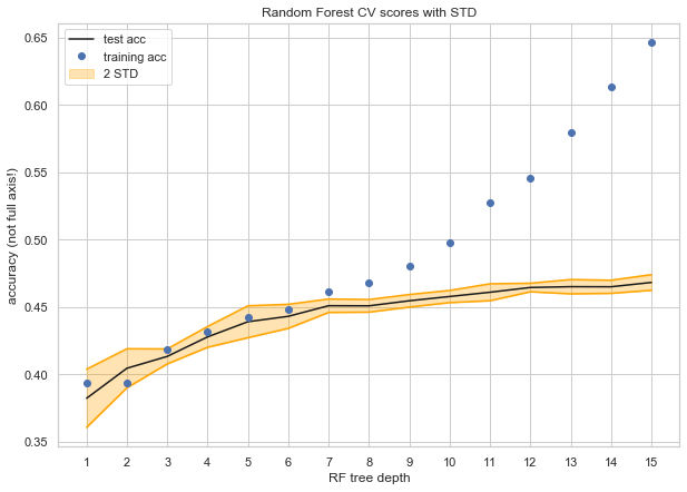
7. Testing for different maximum depths of a Random Forest.


Final Model

The fully documented code for the final model can be found in the final_model.ipynb file. Below is a summary of the model.

A Note About the Baseline Model: to have something to compare to, we looked at what sort of accuracy we would want our model to beat. One way to think of it is the accuracy we would get if responders guessed categories at random (this would be the accuracy given no information about the past). Another way to think about it is the accuracy that a model would produce if it just guessed the most common category 100% of the time (a very naive model). We included both, and decided to compare our model to the latter, because it is more realistic that we do have information about the past when making these decisions.

Our naive baseline accuracy was 20% and our model baseline accuracy was roughly 35.9%.

Set Up the Model: using the knowledge we gained from refining different models, all of which can be found in the folder old_models. From this refining, we decided that the best model would be a Random Forest with a maximum tree depth of 10 (so as to get the best test accuracy without overfitting too much to the training set). We tested each of the hyper parameters that RandomForestClassifier takes, but none helped us improve our accuracy.

Train and Evaluate: the model using the train and test sets. We chose to evaluate our model based on accuracy because other methods didn't make sense. For example, we do care a lot about the false negatives, since not all our categories have the same number of entries, however, since this is not a binary outcome problem, it didn't make sense to use ROC scores. After careful inspection of the class predictions and the predict_proba results, we decided that the accuracy was a good measure of how well our model was performing.

Random Forest Accuracy, Training Set : 50.92%

Random Forest Accuracy, Testing Set : 46.11%

Analysis: as we can see above, our trained model (~50%) performed better than the baseline model (35%). Although the model itself seems simple (we just trained a simple Random Forest on our training data), it is in fact the result of many careful decisions. The real model refining happened in the feature engineering and feature selection process.

Due to the nature of the data (crimes are hard to predict, it can hard to differentiate between a crime that involves drugs or not, and the predictors that we chose cannot possibly capture all the variability in the data), we are confident that our model's accuracy could not significantly improve without drastic changes in the data inputs.

That being said, we wanted to create something that could be useful for a real-life situation, i.e. how can we use the model we created to help emergency responders? The accuracy is pretty low, meaning that given an emergency, the model would only be right about what sort of response was needed 50% of the time. So we decided to use our model to help narrow down the types of responses that could be needed to 2 instead of 5. We could use our model to tell responders "this emergency likely involves drugs and weapons possessions", or "this emergency likely involves domestic issues and drugs". This could help responders send different specialists to each situation, making their response more effective.

In order to accomplish this, we used predict_proba and chose the top two predicted classes for each crime. We used the model trained on the training set, and tested it on the test set to see how good of an accuracy we could get. We were hoping for an accuracy above 75% for a reliable and applicable tool.

Percent of guesses that contained correct category: 74.2 %

Features: As a final useful piece of information, we looked at the most important predictors that help us determine crime type. This could be useful for emergency officials to know for preventative measures. As it turns out, the single most influential feature was the minimum distance to a police station, which is useful to know if considering where to place a new police station.

Most important feature: 'police_min_dist'

Project Trajectory, Results, and Interpretation


Project Trajectory

Our project changed dramatically as we decided what we wanted to focus in on. Overall, we knew we wanted to use the data available to create something that would add value to emergency responders. As we tried to get our model to predict what we thought would be most useful for emergency responders to know, we kept hitting walls with the data, and having to change what we were using our model for, in a way that would still be helpful for our overall question. Usually we wouldn't spend a lot of time on what didn't work--following the quote “people don’t go around introducing you to their ex-wives”--but as this is a school assignment, we wanted to document everything we tried (the model's ex-wives) and how we learned from it.

First, we tried to predict whether a certain crime was a shooting or not (0 or 1). After trying a few models, we soon realized that the number of shootings is too low to accurately predict; our model was simply predicting no shooting for every input, and this gave us high accuracy, but no advantage over the naive model of always predicting the most common outcome, which was no shooting. Even using ROC scores as accuracy, with 1,000 shootings in a 400,000 entry database, we were getting abysmal results.

Next, we tried to predict UCR, the severity of the crime as dictated by the UCR system. This was difficult for a reason similar to the shooting: Part 3 was the most common UCR, so our models were always predicting that. In addition, locational data did not give us that much of an advantage in predicting UCR, since it was distributed somewhat evenly across all the neighborhoods of Boston. The naive model wasn't much worse than the models we could come up with. Also, this was not as useful for our research question, since predicting the UCR did not give much info into the kind of crime being committed, only the severity of said crime.

We then decided that we could predict crime category. Originally we were trying to predict 11 categories of crime, and were making improvements over the naive model. However, our research question made us decide to cut this down to 5 (burglary, violent, possession of weapons, domestic, and drugs), since these could require specialized police units to deal with, and they were the more egregious crimes. This helped us narrow down our research question and produce something that could be helpful in real life.

Throughout all of this experimentation, we documented our model attempts, new EDA, and other tinkering. These can all be found in our project.

Results and Interpretation

From the results shown above in the final model, we see that we can provide a sizable increase over the naive accuracy. If we can predict the top two possibilities of crime with this high of an accuracy, this means we can respond to a crime with the right teams for the job. If police know what kind of crime they are about to see, they can better prepare for it. A violent crime likely to involve weapons should be treated differently than a domestic abuse case involving children. Using our model, we were able to guess the top two most likely crime types with 75% accuracy. This is a step in the right direction for creating a tool that is useful in real life scenarios and helps with resource allocation.

Conclusions and Future Work

Wrap up our findings.


After a few weeks of attempting to predict crime type, we found that it is much more difficult than we anticipated. Crime is a very random event, and where and when it happens can be anywhere and anytime. That being said, we did find some interesting ways to predict the type of crime given some preliminary info, and this could be helpful for police responding quickly and effectively. If we can send specialized law enforcement equipped to handle the top two possibilities as far as type of crime, we can better respond to the situation, possibly saving lives.

In terms of areas where we wish we could have made more progress, data collection comes to mind first. We did our best to brainstorm every type of data that could predict what type of crime would be likely to occur at that time and location, but most of our predictors were very general (neighborhood specific instead of crime location specific) and thus the model had a hard time differentiating between crimes at similar dates and locations. How do you differentiate between a burglary and a drug deal in a similar location on the same day? The other thing we could have benefited from was just more data...if the dataset had gone back more years, then perhaps we could have analyzed how crime types were changing in a specific area and used that to aid predictions. In addition, information about the 911 call would make the model much better (for example, if the 911 call reported a noise disruption in the house next door, then perhaps our model could be trained to predict between burglary and domestic violence, instead of all five categories). All in all, the model performed well, and we learned a lot about feature engineering, and ultimately the model turned out to only be as good as the data we gave it.

CS109A Final Project

by Nicolas Lepore, Natalie Margulies, Daphne Kaxiras, and Wes De Silvestro